understand the distinction between predictive and prescriptive analytics
understand the role of prescriptive analytics within sport
understand the limitations of prescriptive analytics
be familiar with some some common approaches to prescriptive analytics
Note
Remember, this tutorial (like 4.3) is intended to provide you with a general overview of some key ideas and processes that will be covered in more detail in the Research Methods module in Semester Two. There is not need at this stage to fully understand these concepts.
23.2 Introduction
23.2.1 Definition of Prescriptive Analytics
In the previous tutorial, we explored the concept of ‘predictive analytics’. In this tutorial, we’re moving on to think about prescriptive analytics.
Predictive and prescriptive analytics can be thought of as two different approaches to data analytics, each with its own purpose and output. They can be conducted separately, or sequentially, depending on the purpose of your analysis. Usually, they would take place after completing the descriptive analysis.
As we discussed in the previous section, predictive analytics uses statistical techniques to predict future outcomes based on historical data. It answers the question: “What is likely to happen in the future, based on what I already know”?
Predictive analytics doesn’t tell you what action to take, but it can be used to forecast potential outcomes if certain factors are present. For example, it can predict the likelihood of a player getting injured based on current workload and injury history.
In contrast, prescriptive analytics goes a step further than predictive analytics by recommending actions to take for optimal outcomes. It answers the question: “What should we do?”, which is often the thing that coaches, managers and owners are most interested in!
Important
Prescriptive analytics uses techniques such as optimisation, simulation, and decision-tree algorithms to suggest actions that will take advantage of the predictions in your model.
So for example, prescriptive analytics might suggest that a strategy of reducing the player’s training intensity, or increasing rest days, is the best approach. In a business context, it might identify the optimal pricing strategy for season tickets to maximise future sales.
In essence, while predictive analytics forecasts what might happen in the future, prescriptive analytics advises on what actions to take to achieve the best possible outcome.
You may find it helpful to read the following journal article before continuing.
23.3 Development
Prescriptive analytics is a form of advanced analytics that examines data or content to determine what actions should be taken to achieve a particular goal.
It’s distinguished from descriptive analytics, which summarizes raw data and presents it in an understandable form, and predictive analytics, which forecasts future possibilities.
Some potential use-cases for predictive analytics are described below.
23.3.1 Strategic decision-making
Prescriptive analytics can be an invaluable tool for strategic decision-making in sport. It uses algorithms and computational models to suggest the best course of action based on an array of complex data.
For instance, the German soccer team at the 2014 FIFA World Cup worked with SAP to create a match insights software. This prescriptive tool processed data about the team’s tactics and their opponents, helping to inform crucial decisions that ultimately led to their triumph.
23.3.2 Player performance optimisation
Prescriptive analytics also plays a vital role in optimising player performance and maintaining player health. By analysing factors such as player workload, sleep patterns, and biomechanics, sports teams can make proactive decisions to boost performance and prevent injuries.
The Golden State Warriors, an NBA team, used prescriptive analytics to determine the optimum rest days for their players, reducing injuries and enhancing their performance on the court.
23.3.3 Fan engagement
Enhancing the fan experience is another potential application of prescriptive analytics in sports. Sporting organisations can analyse fan behaviour, social media engagement, and ticket sales to provide a more engaging and personalised fan experience.
23.3.4 Challenges and Limitations of Prescriptive Analytics
Despite its potential, prescriptive analytics is not without challenges. Technological barriers, data privacy issues, and the sheer volume and complexity of data can impede implementation. Furthermore, the ethical implications of data collection and use that we’ve discussed before cannot be ignored. IMO, the use of prescriptive analytics should complement, not replace, human judgment and intuition.
23.4 Procedures for Prescriptive Analytics
As noted above, prescriptive analytics builds upon descriptive and predictive analytics to suggest a course of action based on predictions. It involves the application of advanced analytics techniques like optimisation and simulation algorithms, decision-tree models, and complex systems dynamic models, which we will introduce below.
For example, to solve an optimisation problem - finding the best solution from a range of possible solutions - we can use the ‘lpSolve’ package in R to perform linear programming.
In an optimisation problem, you’re basically trying to find the best possible outcome, which could mean getting the highest or lowest result. You do this by picking values from a given set of options and using them in a specific calculation or formula. You keep doing this until you find the best answer
# An example of prescriptive analysis in Rrm(list =ls()) ## create a clean environment# Install the lpSolve package if not installedif(!require(lpSolve)) install.packages('lpSolve')
Here, the code is trying to find the best values for two variables, x1 and x2, so as to get the highest value of the expression 3x1+2x2, but the values chosen must also meet two conditions (constraints) related to how big or small x1 and x2 can be.
23.4.1 Key Components of Prescriptive Analytics
23.4.1.1 Component 1: Optimisation
Optimisation, within the context of prescriptive analytics, is a mathematical approach used to determine the best allocation of limited resources to achieve a specific objective.
The main aim is to maximise desirable factors (like profit, goals scored, or aerobic efficiency) and/or minimize undesirable ones (like injury, points dropped, or waste).
Optimisation models involve three main components:
Decision Variables: These are the variables that the model will determine. For instance, in a sporting context, a decision variable might be the number of hours an athlete should train in a particular skill.
Objective Function: This is the goal that you’re trying to optimise. It might be to maximise something, like team performance, or to minimise something else, like the risk of injury. The objective function is expressed in terms of the decision variables.
Constraints: These are the restrictions or limitations that you need to operate within. They could be based on available resources (like time, money, or personnel), physical or technical restrictions, or specific rules that need to be followed.
The optimisation process involves setting up your model with these three components, and then using mathematical or computational algorithms to find the decision variables that optimise the objective function, subject to the constraints.
Optimisation models are widely used in many fields, including sport. For instance, they might be used to determine the optimal training schedule for an athlete, to maximise performance while minimising the risk of injury, given constraints such as available training time and the need for rest days.
Similarly, in a competitive team sport, optimisation could be used to determine the best combination of players to maximize the team’s overall performance, given constraints like a salary cap and the need to have players in a range of different positions.
23.4.1.2 Component 2: Simulation
Simulation is another powerful tool used in prescriptive analytics that allows decision-makers to model complex scenarios and systems to understand potential outcomes, risks, and opportunities.
It involves the creation of a mathematical model that represents a real-world system, and then running experiments on that model to predict how the system will behave under different circumstances.
Here’s a breakdown of the concept:
Creating a Model: A simulation model represents the key characteristics or behaviors of a selected physical or abstract system. For instance, in sport analytics, a simulation model could represent a basketball game, including player performance statistics, team strategies, and other game-related factors.
Running Experiments: Once the model is created, different scenarios are ‘simulated’ or tested on the model. For example, the impact of different game strategies or player combinations on the outcome of the game can be simulated.
Analysing Results: The results of these simulations are then analyzed to understand potential outcomes, their probabilities, and the factors driving these outcomes. This could include identifying the most successful strategies or player combinations.
Optimisation: Simulation allows for optimisation by identifying the conditions or variables that lead to the best outcome. For instance, it might reveal the optimal player rotation to maximize the team’s scoring potential.
In prescriptive analytics, simulation is used to predict the consequences of different decisions and to suggest the best course of action. It’s particularly useful in situations that are too costly, risky, or time-consuming to experiment in real life, or when there’s a need to make predictions about complex systems with a high degree of uncertainty.
By running simulations, the analyst can gain insights into potential outcomes and make data-informed decisions that optimise results.
23.4.1.3 Component 3: Decision analysis
Decision analysis is a systematic, quantitative, and visual approach to addressing and informing strategic decisions. As a concept within prescriptive analytics, it uses mathematical models, statistical methods, and logic to help decision-makers choose among a set of alternatives.
The primary aim of decision analysis is to provide clarity on the potential outcomes of different choices and to assess their impact on specified goals. It’s especially useful when decisions involve significant complexity or uncertainty.
The process of decision analysis typically involves the following steps:
Identifying the Decision Problem: This includes understanding the decision context, identifying the decision-maker(s), and defining the objectives and constraints.
Structuring the Decision Problem: Decision trees (see below) or influence diagrams are often used to visually represent the problem, showing the possible decision paths, the uncertainties involved, and the potential outcomes.
Identifying Decision Alternatives: These are the different options or courses of action available to the decision-maker.
Developing a Predictive Model: This model uses data and predictive analytics techniques to predict the outcomes of each alternative under various scenarios.
Applying Utility Theory: This involves determining the desirability or value (utility) of the outcomes for the decision-maker, taking into account their risk tolerance and preferences.
Performing the Analysis: The predictive model and utility function are combined to evaluate the alternatives and identify the one that maximizes the expected utility.
Making the Decision: Based on the analysis, the decision-maker can choose the alternative that best meets their objectives.
In the context of sports, for instance, decision analysis can help a team decide whether to draft, trade, or release a player, taking into account the player’s predicted performance, the team’s budget, and the team’s strategic goals.
23.4.1.4 Optional: More on decision trees
Decision trees are a key tool in predictive analytics, and they are used to model the relationships between several input variables and a target variable. In essence, they provide a structured methodology for making decisions based on data.
In the context of predictive analytics, decision trees are used for both classification and regression tasks. A classification tree is used when the outcome is a categorical variable, such as predicting whether a team will win or not. A regression tree, on the other hand, is used when the outcome is a continuous variable, such as predicting the number of points scored.
The decision tree algorithm operates by creating binary splits in the data. At each node of the tree, the algorithm chooses a feature and a split point that best separates the data according to a certain criterion. For classification tasks, this criterion is often the Gini impurity or entropy, which measure the homogeneity of the target variable within the subsets. For regression tasks, the split point is typically chosen to minimise the variance of the target variable within the subsets.
A major advantage of decision trees is their interpretability. The logic of a decision tree can be easily visualized and understood, even by people without a strong background in data science. This makes decision trees a popular choice for applications where interpretability is important, such as credit scoring or medical diagnosis.
However, decision trees also have some limitations. They can easily overfit or underfit the data, so it’s important to tune the complexity of the tree using techniques such as pruning. Decision trees are also sensitive to small changes in the data, which can lead to different splits and potentially different predictions.
Despite these limitations, decision trees are a fundamental building block for more complex models, such as random forests and gradient boosting machines, which use ensemble methods to combine the predictions of multiple decision trees, thereby improving the predictive performance and robustness.
There is more coverage on decision trees, and their implementation in R, below (Section 23.7.1).
23.5 Optimisation Techniques
23.5.1 Introduction
In the context of predictive analytics, ‘optimisation techniques’ refer to the set of methods used to find the best or most efficient solution to a problem, particularly in terms of maximizing or minimizing a particular function.
These methods often involve adjusting the parameters of a predictive model to improve its accuracy or performance.
Here are some key points to understand about optimisation techniques in predictive analytics:
Objective Function: This is the function that needs to be optimised. In predictive analytics, this is often a loss or cost function that measures the discrepancy between the model’s predictions and the actual data. The goal is to minimize this function.
Parameters: These are the variables that the optimisation algorithm changes to minimize or maximize the objective function. In machine learning models, these can include weights and biases in a neural network, or coefficients in a linear regression.
Algorithm: This is the method used to find the optimal parameters. Common optimisation algorithms include gradient descent, stochastic gradient descent, and Newton’s method. More advanced methods include genetic algorithms, simulated annealing, and swarm optimisation.
Constraints: Sometimes, the optimisation problem may have constraints, which are limitations or requirements that the solution must satisfy. For instance, in linear programming, the solution must satisfy a set of linear equality or inequality constraints.
Global vs. Local Optima: Optimisation techniques aim to find the global optimum, which is the best possible solution. However, depending on the shape of the objective function and the algorithm used, they may end up finding a local optimum, which is the best solution in a certain region but not necessarily the best overall solution.
In predictive analytics, optimisation techniques are crucial for training accurate and robust models. They enable the model to learn from data and improve its predictions over time.
23.5.2 Linear programming
23.5.2.1 Introduction
Linear programming is a mathematical method used for determining a way to achieve the best outcome, such as maximum profit or lowest cost, in a given mathematical model for some list of requirements represented as linear equations. It’s a type of optimisation technique used for making the best possible use of available resources.
Here’s a simple overview of Linear Programming:
Objective Function: Linear programming involves the optimisation of a linear objective function, subject to linear equality and inequality constraints. The objective function represents the quantity which needs to be minimized or maximized, such as profit, cost, time, etc.
Decision Variables: These are the variables that decision-makers control and will adjust to optimise the objective function. For instance, in a player recruitment problem, these could be the quantity of different positions to recruit.
Constraints: These are the restrictions or limitations on the decision variables. They form a feasible region within which the solution to the problem lies. Constraints could come from limited resources like materials, labor, or capital, or from requirements such as meeting at least a certain demand for a product.
Solving the Problem: The goal is to find the values of the decision variables that maximize or minimize the objective function while still satisfying the constraints. Graphical methods can be used for problems with two variables. For problems with more than two variables, there are various algorithms, such as the Simplex method and the Interior-Point method.
Feasibility and Optimality: The linear programming problem is said to be feasible if it has some set of values of the decision variables satisfying all the constraints. If the objective function has the best possible (maximum or minimum) value that can be ascribed to it, subject to the constraints, then it is said to have an optimal solution.
Applications: Linear programming can be used in various fields, including business, engineering, economics, and logistics, to optimise resources and operations.
Importantly, linear programming assumes linearity of relationships, which might not always be a realistic assumption. However, despite this limitation, it’s a powerful technique when applicable.
23.5.2.2 Application in sport: Player selection and resource allocation
Let’s imagine we’re an analyst for a professional basketball team, and we’re tasked with optimising the player lineup for the upcoming season. Our objective is to maximize the overall rating of our lineup, subject to a budget constraint (as the team can only afford to pay a certain total amount in player salaries).
For simplicity, let’s assume we’re choosing from 5 players, with the following ratings and salaries:
Player 1: Rating = 85, Salary = £15 million
Player 2: Rating = 92, Salary = £20 million
Player 3: Rating = 88, Salary = £18 million
Player 4: Rating = 80, Salary = £10 million
Player 5: Rating = 83, Salary = £12 million
We’ll also assume that our total budget for player salaries is £50 million.
Here’s how we can solve this problem using the lpSolve package in R:
# Load the lpSolve packagelibrary(lpSolve)# Set the coefficients of the objective functionf.obj <-c(85, 92, 88, 80, 83) # Set the coefficients of the constraintsf.con <-matrix(c(15, 20, 18, 10, 12), nrow=1)# Set the type of constraintsf.dir <-c("<=")# Set the right-hand side coefficientsf.rhs <-c(50)# Run the linear programming modeloptimum_lineup <-lp("max", f.obj, f.con, f.dir, f.rhs, all.bin =TRUE)# Print the optimal solutionprint(optimum_lineup$solution)
[1] 0 1 1 0 1
The lp function is used to define and solve the linear programming problem. The “max” argument indicates that we’re maximizing the objective function. The all.bin = TRUE argument specifies that our decision variables (the players we choose) are binary - in other words, we either choose a player (1) or we don’t (0).
The output of the lp function is a list that includes the optimal values of the decision variables, which can be accessed using optimum_lineup$solution.
In this case, the output will be a vector indicating which players to choose in order to maximize the team’s overall rating while staying within the budget constraint. For example, if the output is (1, 1, 0, 1, 1), this would mean we should choose players 1, 2, 4, and 5.
23.6 Simulation Techniques
Simulation techniques in data analytics involve the use of models to imitate the operation of real-world processes or systems over time.
These techniques allow analysts to make predictions, assess risks, and test hypotheses in a controlled and replicable environment. By adjusting input variables and observing the outcomes, analysts can gain insights into complex phenomena, test scenarios, and optimise decision-making.
Common tools include Monte Carlo simulations, agent-based modeling, and system dynamics, all of which facilitate a deeper understanding of complex systems without the need to interact directly with the ‘real world’.
23.6.1 Monte Carlo simulation
23.6.1.1 What is Monte Carlo Simulation?
Monte Carlo simulation is a computational technique used to model the probability of different outcomes in a process that cannot easily be predicted due to the intervention of random variables. By running simulations many times over, one can calculate the probability of a specific outcome.
In a sporting context, think of it as running a particular game or match 10,000 times in a computer, each time with slightly different variables (e.g., player performances, environmental conditions), and then seeing what percentage of those simulations results in a win, a loss, or a draw.
23.6.1.2 Basic Steps in a Monte Carlo Simulation
Define a model: Understand the problem and the factors influencing the outcome.
Generate random inputs: Use random number generators to produce inputs for the model.
Perform a deterministic computation: Run the model with the random inputs.
Collect and analyze the results: After a large number of iterations, analyze the statistical properties of the outcomes.
23.6.1.3 Monte Carlo Simulation in R
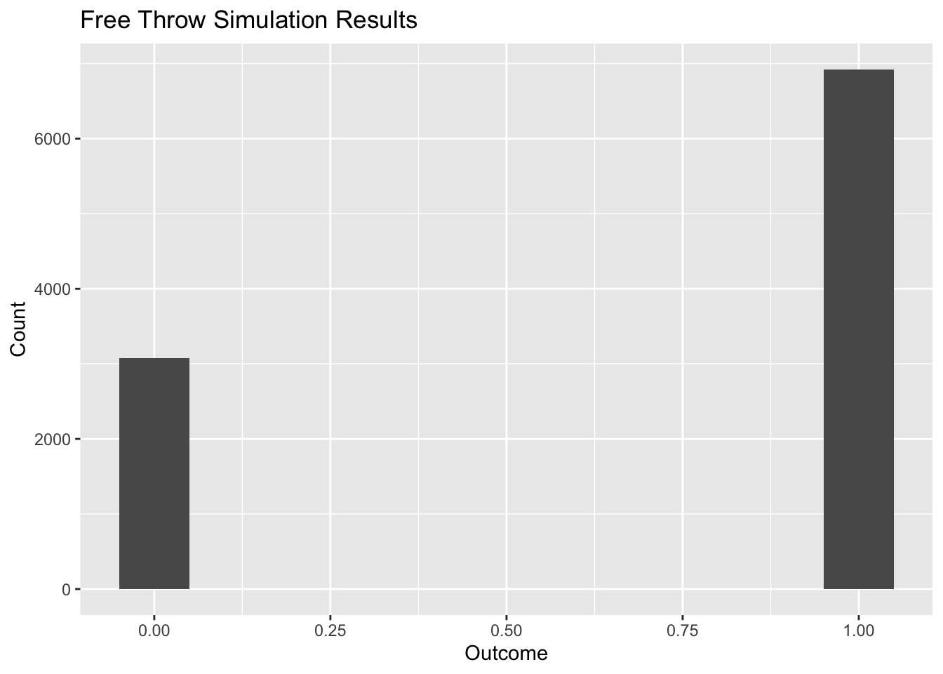
We’ll simulate the outcome of a free throw in basketball. We assume a player has a 70% chance of making a shot.
# Install and load necessary packageslibrary(ggplot2)# Monte Carlo simulation functionsimulate_free_throw <-function(n) { shots_made <-rbinom(n, 1, 0.7)mean(shots_made)}# Run the simulation 10,000 timesn_simulations <-10000results <-replicate(n_simulations, simulate_free_throw(1))# Visualize the resultsdf <-data.frame(success = results)ggplot(df, aes(x = success)) +geom_histogram(binwidth =0.1) +labs(title ="Free Throw Simulation Results", x ="Outcome", y ="Count")
In this example, we can observe that roughly 70% of the outcomes result in a successful shot (or close to that), reinforcing the player’s free throw percentage.
23.6.1.4 Applications in Sports
Monte Carlo simulations can be applied in numerous sports scenarios such as:
Projecting season results: Running a season multiple times to predict which team might win a league or get relegated.
Game strategy optimisation: For instance, understanding the best decisions in high-pressure game situations.
Player performance projections: Predicting how a player might perform over the upcoming season based on various factors.
23.7 Decision Analysis
23.7.1 Decision trees
As we know, sport data analytics involves extracting meaningful insights from vast amounts of sports-related data. It assists teams, athletes, and organizations in making better decisions. One popular tool in this field is the ‘Decision Tree’, a machine learning technique that makes predictions based on asking a series of questions.
A Decision Tree is a flowchart-like structure wherein each node represents a feature (attribute), each branch symbolises a decision rule, and every leaf stands for an outcome. The goal is to create a model that predicts the value of a target variable based on decision rules inferred from data features.
We’ll start with a simple example in R using the rpart package, which is specifically designed for decision trees:
# Install and load necessary packageif(!require(rpart)) install.packages('rpart')
Loading required package: rpart
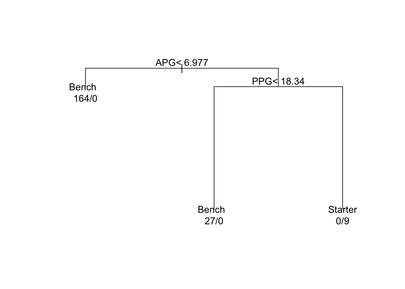
library(rpart)# Generate some mock dataset.seed(123) # To ensure reproducibilityn <-200# Number of playersPPG <-rnorm(n, mean=15, sd=5)APG <-rnorm(n, mean=5, sd=2)Role <-ifelse(PPG >=18& APG >=7, "Starter", "Bench")players_data <-data.frame(PPG, APG, Role)# Create the Decision Treetree_model <-rpart(Role ~ PPG + APG, data=players_data, method="class")# Print the decision tree summaryprint(tree_model)
# Visualize the treeplot(tree_model, margin=0.1)text(tree_model, use.n=TRUE)
This decision tree classifies 200 players into two roles: “Starter” and “Bench”. Here’s a basic interpretation of the tree’s outcome:
If a player’s average points per game (PPG) are equal to or greater than a certain threshold, say 18, the tree might further check the player’s average assists per game (APG).
Among those with high PPG, if their APG is also above a certain level, say 7, they are likely to be classified as a “Starter”. If not, they might still be placed on the bench.
Players with PPG below the initial threshold are more often than not categorized as “Bench” players, regardless of their APG.
This decision tree suggests that while both PPG and APG are important, a player’s scoring ability (PPG) is the primary factor determining their role. However, when PPG is high, their playmaking ability (APG) can further influence the decision.
In this example, we have trained our model on the entire dataset. Usually, we prefer to split our model into training and testing sub-sets.
As you can likely see, decision trees can be used in numerous applications in sport, including:
Talent Identification: By examining a variety of metrics (like speed, strength, agility, and game statistics), decision trees can help in identifying potential talents in junior leagues or academies.
Injury Prediction: Using data from training, health metrics, and past injury records, decision trees can be utilised to predict the likelihood of a player getting injured.
Game Strategy: Based on historical game data, decision trees might suggest, for instance, if a basketball team should attempt a 3-point shot or drive to the basket based on game context (e.g., score difference, time remaining).
Ticket Sales Prediction: Factors like team performance, opponent popularity, and day of the week can be used in decision trees can help lubs anticipate ticket sales for upcoming matches, aiding in marketing strategies.
There’s an interesting step-by-step description of building a decision tree in sport here. The author uses Python rather than R, but the steps and interpretation are the same.